3 Solving Problems By Searching

3.1 Problem-solving Agents

Problem-solving agents

A problem-solving agent is a specialized type of goal-based agent.
It uses atomic representations for the state space.

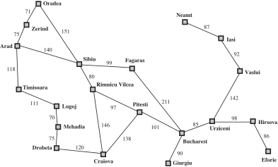
Example: Romania travelling

You are currently located in Arad.
You must attend a friend’s wedding in Bucharest tomorrow.

Properties of the environment

Observable
- The agent always knows the current state (e.g., each city has a sign indicating its presence).
Discrete
- There are a finite number of actions available from any given state (e.g., each city connects to a small number of other cities).
Known
- The agent understands the consequences of each action (i.e., which states are reached).
Deterministic
- Each action results in exactly one outcome.
- Under these assumptions, the solution to any problem is a fixed sequence of actions.

Solving problems by searching

Search: The process of looking for a sequence of actions that reaches the goal.
- A search algorithm takes a problem as input and returns a solution in the form of an action sequence.
Execution phase: Once a solution is found, the recommended actions are carried out.
- While executing the solution, the agent ignores its percepts when choosing an action, operating as an open-loop system.

function Simple-Problem-Solving-Agent(percept) returns an action

persistent: seq: an action sequence, initially empty
           state: some description of the current world state
           goal: a goal, initially null
           problem: a problem formulation

  state ← Update-State(state, percept)

  if seq is empty then
    goal ← Formulate-Goal(state)
    problem ← Formulate-Problem(state, goal)
    seq ← Search(problem)
    if seq = failure then return a null action
  
  action ← First(seq)
  seq ← Rest(seq)

return action

Well-defined problems and solutions

A problem can be formally defined by five components:

The initial state that the agent starts in.
- For example, the initial state for our agent in Romania might be described as In(Arad).
A description of the possible actions available to the agent.
- For example, Action(In(Arad)) = {Go(Sibiu), Go(Timisoara), Go(Zerind)}.
The transition model, which describes what each action does.
- For example, Result(In(Arad), Go(Zerind)) \to In(Zerind).
- We use the term successor to refer to any state reachable from a given state by a single action.
- The initial state, actions, and transition model implicitly define the state space of the problem.
- The state space forms a directed network or graph in which the nodes are states and the links between nodes are actions.
- A path in the state space is a sequence of states connected by a sequence of actions.
The goal test, which determines whether a given state is a goal state.
- For example, the agent’s goal in Romania is the singleton set {In(Bucharest)}.
A path cost function that assigns a numeric cost to each path.
- The step cost of taking action a in state s to reach state s’ is denoted by c(s, a, s’).

A solution to a problem is an action sequence that leads from the initial state to a goal state.

An optimal solution has the lowest path cost among all solutions.

Formulating problems by abstraction

Abstraction is the process of removing detail from a representation, specifically by simplifying the state description and the actions.
Abstraction is critical for automated problem solving because:
- The real world is often too detailed to model exactly.
- We must create an approximate, simplified model of the world for the computer to process.
The choice of a good abstraction involves:
- Removing as much detail as possible, while
- Retaining validity and ensuring that the abstract actions are feasible to carry out.

Directed Graphs

A directed graph G=(V,E) consists of a set V of nodes and a set E of ordered pairs of nodes, called arcs.

3.2 Example Problems

Toy problems vs. Real-world problems

Toy problems	Real-world problems
Illustrate or exercise various problem- solving methods	More difficult
Concise, exact description	No single, agreed-upon description
Can be used to compare performance
E.g., 8-puzzle, 8-queens problem, Cryptarithmetic, Vacuum world, Missionaries and cannibals, simple route finding	E.g., Route finding, Touring and traveling salesperson problems, VLSI layout, Robot navigation, Assembly sequencing

The vacuum world

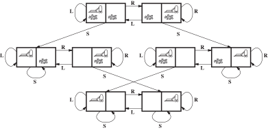
States: The state is determined by both the agent’s location and the dirt locations. Thus, there are 2\times2^{2}=8 possible world states (n\times2^{n} states in general).

Initial state: Any state can be designated as the initial state.
Actions: In this simple environment, each state has just three actions: Left, Right, and Suck. Larger environments might also include Up and Down.
Goal test: This checks whether all the squares are clean.
Path cost: Each step costs 1.
Transition model: State space.

The 8-puzzle

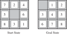
States: A state description specifies the location of each of the eight tiles and the blank space in one of the nine squares.

Initial state: Any state can be designated as the initial state.
Actions:
- Left, Right, Up, or Down.
- Different subsets of these are possible depending on the position of the blank space.
Transition model: Given a state and action, this returns the resulting state.
Goal test: This checks whether the state matches the goal configuration.
Path cost: Each step costs 1.

It is a member of the family of sliding-block puzzles and is NP-complete.
8-puzzle: 9!/2 = 181,440 reachable states \rightarrow easily solved.
15-puzzle (on a 4\times4 board): 1.3 trillion states \rightarrow optimally solved in a few milliseconds.
24-puzzle (on a 5\times5 board): around 10^{25} states \rightarrow optimally solved in several hours.

The 8-queens

There are two main approaches to formulation:

An incremental formulation involves operators that augment the state description, starting with an empty state; for the 8-queens problem, each action adds a queen to the board.
A complete-state formulation starts with all 8 queens on the board and moves them around.

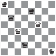
Incremental formulation:

States: Any arrangement of 0 to 8 queens on the board constitutes a state.
- The number of states is 64\times63\ldots57\approx1.8\times10^{14}.
Initial state: No queens on the board.
Actions: Add a queen to any empty square.
Transition model: Returns the board with a queen added to the specified square.
Goal test: 8 queens are on the board, with none attacking another.
Path cost: Irrelevant (we are only interested in the final state).

Pacman

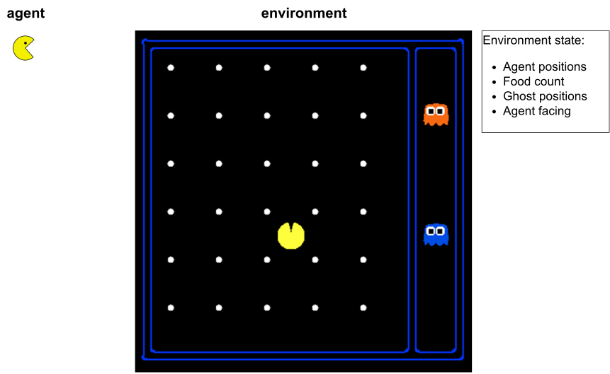
Knuth’s 4 problem

Devised by Donald Knuth (1964).

This illustrates how infinite state spaces can arise.
Knuth’s conjecture: Starting with the number 4, a sequence of factorial \cdot!, square root \sqrt{\cdot}, and floor \lfloor \cdot\rfloor operations can reach any desired positive integer.

\left\lfloor \sqrt{\sqrt{\sqrt{\sqrt{\sqrt{(4!)!}}}}}\right\rfloor =5

States: Any positive number.

Initial state: 4.
Actions: Apply factorial, square root, or floor operation.
Transition model: Defined by the mathematical definitions of the operations (factorial applies to integers only).
Goal test: The state matches the desired positive integer.

The route-finding problem

Consider the airline travel problems solved by a travel-planning website.

States: Each state includes a location (e.g., an airport) and the current time.

Initial state: Specified by the user’s query.
Actions: Take any flight from the current location, in any seat class, leaving after the current time, provided there is enough time for within-airport transfer.
Transition model: The state resulting from taking a flight has the flight’s destination as the current location and the flight’s arrival time as the current time.
Goal test: Are we at the final destination specified by the user?
Path cost: This depends on monetary cost, waiting time, flight time, customs and immigration procedures, seat quality, time of day, airplane type, frequent-flyer mileage awards, etc.

Example: robotic assembly

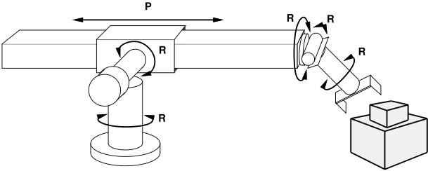
States: Real-valued coordinates of robot joint angles and parts of the object to be assembled.
Actions: Continuous motions of robot joints.
Goal test: Complete assembly with no robot included!
Path cost: Time required to execute.

3.3 Searching for Solutions

Search tree

Since a solution is an action sequence, search algorithms work by considering various possible action sequences.

Search tree: This represents the possible action sequences starting at the initial state.
- The branches correspond to actions, and the nodes correspond to states in the state space of the problem.
- The root node of the tree corresponds to the initial state.
- Actions are taken by expanding the current state (parent node), thereby generating a new set of states (child nodes).
- Frontier: The set of all leaf nodes available for expansion at any given point.

Search algorithms all share this basic structure; they vary primarily according to how they choose which state to expand next—the so-called search strategy.

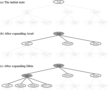
Partial search trees for finding a route from Arad to Bucharest. Nodes that have been expanded are shaded; nodes that have been generated but not yet expanded are outlined in bold; nodes that have not yet been generated are shown in faint dashed lines.

function Tree-Search(problem) returns a solution, or failure

  initialize the frontier using the initial state of problem

  loop do
    if the frontier is empty then
      return failure
    choose a leaf node and remove it from the frontier
    if the node contains a goal state then
      return the corresponding solution
    expand the chosen node, adding the resulting nodes to the frontier

Redundant paths

Loopy paths cause repeated states in the search tree.

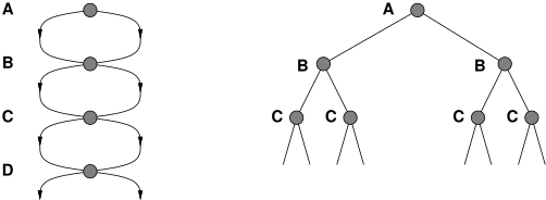
Redundant paths (a general concept) are unavoidable and exist whenever there is more than one way to get from one state to another.
Following redundant paths can cause a tractable problem to become intractable.
This is true even for algorithms that know how to avoid infinite loops.

Graph search algorithm

Algorithms that forget their history are doomed to repeat it.
To avoid redundancy, we use a data structure called the explored set, which remembers every expanded node.

function Graph-Search(problem) returns a solution, or failure

  initialize the frontier using the initial state of problem
  initialize the explored set to be empty

  loop do
    if the frontier is empty then
      return failure
    choose a leaf node and remove it from the frontier
    if the node contains a goal state then
      return the corresponding solution
    add the node to the explored set
    expand the chosen node,
      adding the resulting nodes to the frontier
      only if not in the frontier or explored set

The algorithm has another important property: the frontier separates the state-space graph into the explored region and the unexplored region. Every path from the initial state to an unexplored state must pass through a state in the frontier.

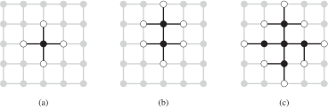
The frontier (white nodes) always separates the explored region of the state space (black nodes) from the unexplored region (gray nodes).

Infrastructure for search algorithms

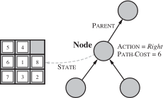
Search algorithms require a data structure to track the search tree being constructed. For each node n of the tree, we use a structure containing four components:

n.State: The state in the state space to which the node corresponds.
n.Parent: The node in the search tree that generated this node.
n.Action: The action that was applied to the parent to generate the node.
n.PathCost: The cost, traditionally denoted by g(n), of the path from the initial state to the node, as indicated by the parent pointers.

function Child-Node(problem, parent, action) returns a node

  return a node with
    State ← problem.Result(parent.State, action),
    Parent ← parent,
    Action ← action,
    Path-Cost ← parent.Path-Cost + problem.Step-Cost(parent.State, action)

Measuring problem-solving performance

We can evaluate an algorithm’s performance in four ways:

Completeness: Is the algorithm guaranteed to find a solution when there is one?
Optimality: Does the strategy find the optimal solution?
Time complexity: How long does it take to find a solution?
Space complexity: How much memory is needed to perform the search?

Time and space complexity are measured in terms of:

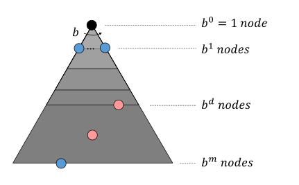
b: Maximum branching factor of the search tree.
d: Depth of the least-cost/shallowest solution.
m: Maximum depth of the state space (may be \infty).