8 Adversarial Search
Adversarial Search
- Multiagent environments: each agent needs to consider the actions of other agents and how they affect its own welfare.
- Competitive environments: the agents’ goals are in conflict, giving rise to adversarial search problems, often known as games
- The unpredictability of other agents introduce contingencies into the agent’s problem-solving process.
Types of Games
- Many different kinds of games!
- Axes:
- Deterministic or stochastic?
- One, two, or more players?
- Zero sum?
- Perfect information (can you see the state)?
- Want algorithms for calculating a strategy (policy) which recommends a move from each state
| deterministic | chance | |
|---|---|---|
| perfect information | chess, checkers, go, othello | backgammon, monopoly |
| imperfect information | battleships, blind tic-tac-toe | bridge, poker, scrabble nuclear war |
Deterministic Games
A game can be formally defined as a kind of search problem with the following elements:
- S_{0}: The initial state, which specifies how the game is set up at the start.
- Player(): Defines which player has the move in a state.
- Actions(s): Returns the set of legal moves in a state.
- Result(a): The transition model, which defines the result of a move.
- Terminal-test(s): A terminal test, which is true when the game is over and false otherwise. States where the game has ended are called terminal states.
- Utility(p): A utility function(also called an objective function or payoff function), defines the final numeric value for a game that ends in terminal states for a player
Zero-Sum Games
- Zero-Sum Games
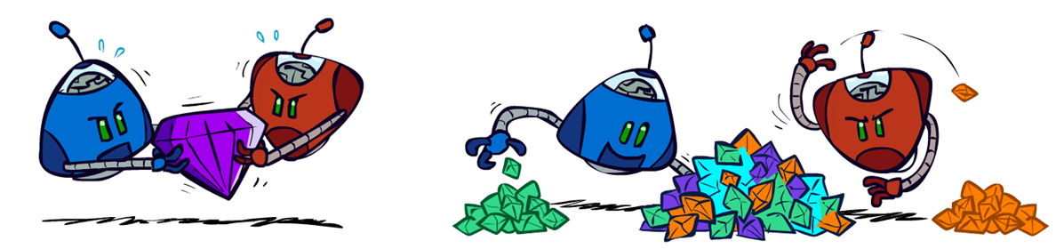
- Agents have opposite utilities (values on outcomes)
- Lets us think of a single value that one maximizes and the other minimizes
- Adversarial, pure competition
- General Games
- Agents have independent utilities (values on outcomes)
- Cooperation, indifference, competition, and more are all possible
We consider the game
- Two players only, called MAX and MIN.
- MAX moves first, and then they take turns moving until the game
- Winner gets reward, loser gets penalty.
- Both players have complete knowledge of the game’s state
- E.g., chess, checkers and Go, etc. Counter examples: poker
- No element of chance
- No dice thrown, no cards drawn, etc.
- Zero-sum games
- The total payoff to all players is the same for every game instance.
- Rational players
- Each player always tries to maximize his/her utility
Game tree
- The initial state, Actions function, and Result function define the game tree where the nodes are game states and the edges are moves
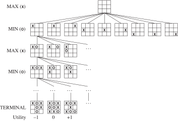
A (partial) game tree for the game of tic-tac-toe.
8.1 State-Of-The-Art Game Programs
Checkers
- Complexity
- \approx10^{18}nodes, which may require 100k years with 106 positions/sec
- Chinook (1989-2007)
- The first computer program to win the world champion title in a competition against humans.
- 1990: won 2 games in competition with world champion Tinsley (final score: 2 - 4, 33 draws)
- 1994: 6 draws
- Chinook’s search
- Ran on regular PCs, play perfectly by using alpha-beta search combining with a database of 39 trillion endgame positions
Chess
- Complexity
- b\approx35, d\approx100, 10^{154} nodes
- Completely impractical to search this
- Deep Blue (May 11, 1997)
- Kasparov lost a 6-game match against IBM’s Deep Blue (1 win Kasp – 2 wins DB) and 3 ties.
- In the future, focus will be to allow computers to LEARN to play chess rather than being TOLD how it should play
Go
- Complexity
- Board of 19\times19, b\approx361, average depth 200
- 10^{174} possible board configuration.
- Control of territory is unpredictable until the endgame
- AlphaGo (2016) by Google
- Beat 9-dan professional Lee Sedol (4 - 1)
- Machine learning + Monte Carlo search guided by a “value network” and a “policy network” (implemented using deep neural network technology)
- Learn from human + Learn by itself (self-play games)
8.2 Optimal Decisions in Games
Optimal decisions in games
- Normal search problem
- Optimal solution is a sequence of action leading to a goal state.
- Games
- A search path that guarantee win for a player
- The optimal strategy can be determined from the minimax value of each node
\text{Minimax}(s)=\left\{ \begin{array}{ll} \text{Utility}(s) & \text{if}\;\text{Terminal-Test}(s)\\ \max_{a\in\text{Actions}(s)}\text{Minimax}(\text{Result}(s,a)) & \text{if}\;\text{Player}(s)=MAX\\ \min_{a\in\text{Actions}(s)}\text{Minimax}(\text{Result}(s,a)) & \text{if}\;\text{Player}(s)=MIN \end{array}\right.
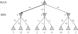
A two-player game tree. The \Delta nodes are MAX nodes, in which it is MAX’s turn to move, and the \nabla nodes are MIN nodes. The terminal nodes show the utility values for MAX; the other nodes are labeled with their minimax values.
The minimax algorithm
- Compute the minimax decision from the current state
- Use a simple recursive computation of the minimax values of each successor state
- The recursion proceeds all the way down to the leaves of the tree, and then the minimax values are backed up through the tree as the recursion unwinds.
function Minimax-Decision(state) returns an action
    bestAction ← null
    bestValue ← −∞

    for each a in Actions(state) do
        value ← Min-Value(Result(state, a))
        if value > bestValue then
            bestValue ← value
            bestAction ← a

    return bestAction

function Max-Value(state) returns a utility value
    if Terminal-Test(state) then
        return Utility(state)

    v ← −∞
    for each a in Actions(state) do
        v ← Max(v, Min-Value(Result(state, a)))

    return v

function Min-Value(state) returns a utility value
    if Terminal-Test(state) then
        return Utility(state)

    v ← +∞
    for each a in Actions(state) do
        v ← Min(v, Max-Value(Result(state, a)))

    return v
Properties
A complete depth-first exploration of the game tree
- Completeness
- Yes (if tree is finite)
- Optimality
- Yes (against an optimal opponent)
- Time complexity: O(b^{m})
- Space complexity: O(bm) (depth-first exploration)
For chess, b\approx35, m\approx100 for ``reasonable’’ games \Rightarrow exact solution completely infeasible
But do we need to explore every path?
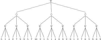
Exercise
- Calculate the utility values for the remaining nodes of the game tree
Optimal decisions in multiplayer games
- A single value is replaced with a vector of values
- the Utility function return a vector of utilities
- For terminal states, this vector gives the utility of the state from each player’s viewpoint.
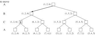
The first three plies of a game tree with three players (A, B, C). Each node is labeled with values from the viewpoint of each player. The best move is marked at the root.
- Challenges in multiplayer games
- Multiplayer games usually involve alliances, which are made and broken as the game proceeds.
- If the game is not zero-sum, then collaboration can also occur with just two players.
8.3 Alpha–Beta Pruning
Problem with minimax search
- The number of game states is exponential in the tree’s depth
- Do not examine every node
- Alpha-beta pruning: Prune away branches that cannot possibly influence the final decision
- Bounded lookahead
- Limit depth for each search
- This is what chess players do: look ahead for a few moves and see what looks best
Trick to compute
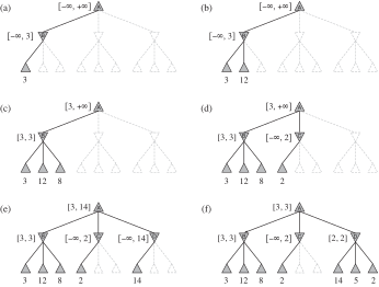
\begin{align*} \text{Minimax}(root) & =\max(\min(3,12,8),\min(2,x,y),\min(14,5,2))\\ & =\max(3,\min(2,x,y),2)\\ & =\max(3,z,2)\hspace*{1em}\text{where}\:z=\min(2,x,y)\leq2\\ & =3 \end{align*}
Alpha-beta pruning
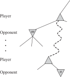
The general case for alpha-beta pruning. If m is better than n for Player, we will never get to n in play.
Minimax search is depth-first, so at any one time we just have to consider the nodes along a single path in the tree. Alpha-beta pruning has the two parameters that describe bounds on the backed-up values that appear anywhere along the path
- \alpha = the value of the best (i.e., highest-value) choice we have found so far at any choice point along the path for MAX.
- \beta = the value of the best (i.e., lowest-value) choice we have found so far at any choice point along the path for MIN.
The alpha-beta search algorithm
function Alpha-Beta-Search(state) returns an action
    α ← −∞
    β ← +∞
    bestAction ← null
    bestValue ← −∞

    for each a in Actions(state) do
        value ← Min-Value(Result(state, a), α, β)
        if value > bestValue then
            bestValue ← value
            bestAction ← a
        α ← Max(α, bestValue)

    return bestAction

function Max-Value(state, α, β) returns a utility value
    if Terminal-Test(state) then
        return Utility(state)

    v ← −∞
    for each a in Actions(state) do
        v ← Max(v, Min-Value(Result(state, a), α, β))
        if v ≥ β then
            return v
        α ← Max(α, v)

    return v

function Min-Value(state, α, β) returns a utility value
    if Terminal-Test(state) then
        return Utility(state)

    v ← +∞
    for each a in Actions(state) do
        v ← Min(v, Max-Value(Result(state, a), α, β))
        if v ≤ α then
            return v
        β ← Min(β, v)

    return v
Properties
- Pruning does not affect final result
- Pruning can reduce the tree size while its worst case is as good as the minimax algorithm
- Good move ordering improves effectiveness of pruning
- With perfect ordering’’, time complexity O(b^{m/2}) \Rightarrow doubles solvable depth
- In chess, Deep Blue achieved depth reduction from 38 to 6
- Killer move heuristic
- First, IDS search with 1 ply deep and record the best path. Then search 1 ply deeper with the recorded path to inform move ordering.
- Transposition table avoids re-evaluation a state
8.4 Imperfect Real-time Decisions
Evaluation functions
- Both minimax and alpha-beta pruning search all the way to terminal states
- This depth is usually not practical because moves must be made in a reasonable amount of time (~ minutes).
- Cut off the search earlier with some depth limit
- Use an evaluation function Eval
- An estimation for the desirability of position (win, lose, tie?)
\text{H-Minimax}(s,d)=\left\{ \begin{array}{ll} \text{Eval}(s) & \text{if}\;\text{Cutoff-Test}(s,d)\\ \max_{a\in\text{Actions}(s)}\text{H-Minimax}(\text{Result}(s,a),d+1) & \text{if}\;\text{Player}(s)=MAX\\ \min_{a\in\text{Actions}(s)}\text{H-Minimax}(\text{Result}(s,a),d+1) & \text{if}\;\text{Player}(s)=MIN \end{array}\right.
The evaluation function should order the terminal states in the same way as the true utility function does
- States that are wins must evaluate better than draws, which in turn must be better than losses.
The computation must not take too long!
For nonterminal states, the evaluation function should be strongly correlated with the actual chances of winning
For chess, typically linear weighted sum of features \text{Eval}(s)=w_{1}f_{1}(s)+w_{2}f_{2}(s)+\ldots+w_{n}f_{n}(s)=\sum_{i=1}^{n}w_{i}f_{i}(s) where each w_{i} is a weight and each f_{i} is a feature of each kind of piece (move number or* number of remaining pieces*)
Implicit strong assumption: the contribution of each feature is independent of the values of the other features.
Current programs for chess and other games also use nonlinear combinations of features
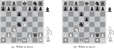
Two chess positions that differ only in the position of the rook at lower right. In (a), Black has an advantage of a knight and two pawns, which should be enough to win the game. In (b), White will capture the queen, giving it an advantage that should be strong enough to win.
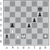
The horizon effect. With Black to move, the black bishop is surely doomed. But Black can forestall that event by checking the white king with its pawns, forcing the king to capture the pawns. This pushes the inevitable loss of the bishop over the horizon, and thus the pawn sacrifices are seen by the search algorithm as good moves rather than bad ones.
Cutting off search
Cuttingoff-Search is almost identical to Alpha-Beta-Search except
- Terminal-Test is replace by Cutoff-Test
- Utility is replaced by Eval
if Cutoff-Test (state, depth) then return Eval(state)
- The depth is incremented on each recursive call
- Cutoff-Test(state, depth) returns true for all depth greater than some fixed depth d
How to improve?
- Using a more sophisticated cutoff test
- Quiescent positions are those unlikely to exhibit wild swings in value in the near future.
- Quiescence search: Expand nonquiescent positions until quiescent positions are reached.
- Beam search
- Forward pruning, consider only a “beam” of the n best moves only
- Most humans consider only a few moves from each position
- PROBCUT, or probabilistic cut, algorithm (Buro, 1995)
- Search vs. lookup
- Use table lookup rather than search for the opening and ending
8.5 Stochastic Games
Stochastic behaviors
- Uncertain outcomes controlled by chance, not an adversary!
- Why wouldn’t we know what the result of an action will be?
- Explicit randomness: rolling dice
- Unpredictable opponents: the ghosts respond randomly
- Actions can fail: when moving a robot, wheels might slip
Expectimax Search Trees
- A game tree must include chance nodes in addition to MAX and MIN nodes
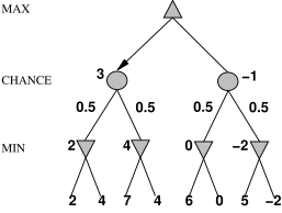
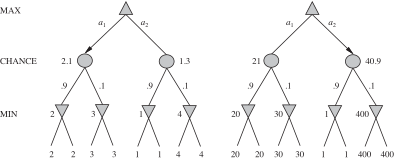
Chance nodes introduced by fair coin-flipping
Expectimax search
- Values should now reflect average-case (expectimax) outcomes, not worst-case (minimax) outcomes
- Expectimax search:
- MAX/MIN nodes as in minimax search
- CHANCE nodes: we compute the expected value, which is the sum of the value over all outcomes, weighted by the probability of each chance action
- The underlying uncertain-result problems can be formulated as Markov Decision Processes
\text{Expectiminimax}(s)=\left\{ \begin{array}{ll} \text{Utility}(s) & \text{if}\;\text{Terminal-Test}(s)\\ \max_{a\in\text{Actions}(s)}\text{Expectiminimax}(\text{Result}(s,a)) & \text{if}\;\text{Player}(s)=MAX\\ \min_{a\in\text{Actions}(s)}\text{Expectiminimax}(\text{Result}(s,a)) & \text{if}\;\text{Player}(s)=MIN\\ \sum_{r}P(r)\text{Expectiminimax}(\text{Result}(s,r)) & \text{if}\;\text{Player}(s)=CHANCE \end{array}\right.
Expectimax Pruning?
- Not easy
- exact: need bounds on possible values
- approximate: sample high-probability branches
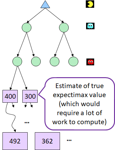
Depth-Limited Expectimax
Evaluation functions for games of chance
Minimax:
- Exact values don’t matter
- Behaviour is preserved under any monotonic transformation of
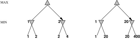
Expectimax:
- Exact values DO matter
- Behaviour is preserved only by positive linear transformation of