4 Uninformed search strategies
- These strategies possess no additional information about states beyond what is provided in the problem definition.
- They can only generate successors and distinguish a goal state from a non-goal state.
- They are also referred to as blind search.
- Each strategy is a modified instance of the general tree/graph search algorithm.
4.1 Breadth-first search
Breadth-first search
- Breadth-first search (BFS) is a simple strategy in which the root node is expanded first, followed by all successors of the root node, then their successors, and so on.
- In generally, all nodes at a given depth in the search tree are expanded before any nodes at the next level.
- Breadth-first search on a simple binary tree. At each stage, the node to be expanded next is indicated by a marker.

Algorithm
- The frontier is implemented as a FIFO queue.
function Breadth-First-Search(problem) returns a solution, or failure

  node ← a node with State = problem.Initial-State, Path-Cost = 0
  if problem.Goal-Test(node.State) then return Solution(node)
  frontier ← node
  explored ← ⌀
  loop do
    if frontier = ⌀ then return failure
    node ← Pop(frontier)
    add node.State to explored
    for each action in problem.Actions(node.State) do
      child ← Child-Node(problem,node,action)
      if child.State is not in explored or frontier then
        if problem.Goal-Test(child.State) then return Solution(child)
        frontier ← Insert(child,frontier)
Properties of breadth-first search
- Time: 1+b+b^{2}+b^{3}+\ldots+b^{d}=O(b^{d})
- Space: O(b^{d}) (O(b^{d-1}) for explored and O(b^{d}) for frontier)
- Complete: Yes (if b is finite)
- Optimal: Not optimal in general (unless step costs are identical)
| Depth | Nodes | Time | Memory |
|---|---|---|---|
| 2 | 110 | .11 milliseconds | 107 kilobytes |
| 4 | 11,110 | 11 milliseconds | 10.6 megabytes |
| 6 | 10^{6} | 1.1 seconds | 1 gigabyte |
| 8 | 10^{8} | 2 minutes | 103 gigabytes |
| 10 | 10^{10} | 3 hours | 10 terabytes |
| 12 | 10^{12} | 13 days | 1 petabyte |
| 14 | 10^{14} | 3.5 years | 99 petabytes |
| 16 | 10^{16} | 350 years | 10 exabytes |
Time and memory requirements for breadth-first search. The numbers shown assume branching factor b = 10; 1 million nodes/second; 1000 bytes/node.
4.2 Uniform-cost search
Uniform-cost search
- Uniform-cost search (UCS) expands the node n with the lowest path cost g(n).
- Implementation: The frontier is a priority queue ordered by g.
- This is equivalent to Dijkstra’s algorithm.
- The goal test is applied to a node only when it is selected for expansion.
- A test is added in case a better path is found to a node currently on the frontier.
Algorithm
- The frontier is a priority queue.
function Uniform-Cost-Search(problem) returns a solution, or failure

  node ← a node with State = problem.Initial-State, Path-Cost = 0
  frontier ← node // a priority queue ordered by Path-Cost
  explored ← ⌀
  loop do
    if frontier = ⌀ then return failure
    node ← Pop(frontier) // chooses the lowest-cost node in frontier
    if problem.Goal-Test(node.State) then return Solution(node)
    add node.State to explored
    for each action in problem.Actions(node.State) do
      child ← Child-Node(problem,node,action)
      if child.State is not in explored or frontier then
        frontier ← Insert(child,frontier)
      else if child.State is in frontier with higher Path-Cost then
        replace that frontier node with child
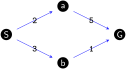
A critical question arises: Should we apply the goal test when we enqueue a node or when we dequeue it?
Find a path from S to G
Properties of uniform-cost search
- Time: O(b^{1+\left\lfloor \frac{C^{*}}{\epsilon}\right\rfloor }) where C^{*} is the cost of the optimal solution
- Space: O(b^{1+\left\lfloor\frac{C^{*}}{\epsilon}\right\rfloor})
- Complete: Yes, if step cost \geq\epsilon (where \epsilon is a small positive constant)
- Optimal: Yes, nodes are expanded in increasing order of g(n)
Proof (by contradiction)
- Suppose UCS terminates at a goal state n with a path cost g(n)=C.
- If C is not the optimal value, then there exists another unexplored goal state n' with g(n')<C.
- Therefore, there must exist a node n'' on the frontier that is on the optimal path to n' (graph separation property).
- However, g(n'')<g(n')<g(n) implies that n'' must be expanded before n, which is a contradiction.
Ilustration
Find a shortest path from a to f

Step-by-step execution


| node | frontier |
|---|---|
| a(0;null) | |
| a(0;null) | b(9;a) d(3;a) g(6;a) |
| d(3;a) | b(7;d) g(6;a) c(4;d) e(11;d) |
| c(4;d) | b(7;d) g(6;a) e(9;c) |
| g(6;a) | b(7;d) e(9;c) |
| b(7;d) | e(9;c) |
| e(9;c) | f(26;e) |
| f(26;e) | \emptyset |
4.3 Depth-first search
Depth-first search
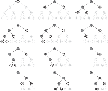
- Depth-first search (DFS) expands the deepest unexpanded node first.
- Implementation: The frontier is a LIFO (Last-In-First-Out) Stack.
- Depth-first search on a binary tree. The unexplored region is shown in light gray. Explored nodes with no descendants in the frontier are removed from memory. Nodes at depth 3 have no successors and M is the only goal node.
Properties of DFS
- Time: O(b^{m})
- Performance is poor if m is significantly larger than d, but if solutions are dense, it may be much faster than breadth-first search.
- Space: O(bm), i.e., linear space!
- Complete:
- No in infinite-depth spaces.
- Yes in finite spaces.
- Optimal: No, it finds the “leftmost” solution, regardless of depth or cost.
4.4 Depth-limited search
Depth-limited Search
- Depth-limited Search (DLS) is a standard DFS with a predetermined depth limit l; nodes at depth l are treated as if they have no successors.
- This allows infinite problems to be solved (by imposing a finite limit).
- Depth limits can be chosen based on prior knowledge of the problem.
Algorithm
- A recursive implementation of depth-limited tree search.
function Depth-Limited-Search(problem,limit) returns a solution, or failure/cutoff

  return Recursive-Dls(Make-Node(problem.Initial-State),problem,limit)

function Recursive-Dls(node,problem,limit) returns a solution, or failure/cutoff

  if problem.Goal-Test(node.State) then return Solution(node)
  else if limit = 0 then return cutoff
  else
    cutoff_occurred? ← false
    for each action in problem.Actions(node.State) do
      child ← Child-Node(problem,node,action)
      result ← Recursive-Dls(child,problem,limit-1)
      if result = cutoff then cutoff_occurred? ← true
      else if result ≠ failure then return result
    if cutoff_occurred? then return cutoff
    else return failure
Properties
- Time
- O(b^{l})
- Space
- O(bl)
- Completeness
- May be incomplete if l<d (the goal is deeper than the limit).
- Optimal: Not optimal if l>d.
4.5 Iterative deepening depth-first search
Iterative deepening depth-first search
- This is a general strategy, often used in combination with depth-first tree search to find the best depth limit.
- It works by gradually increasing the limit until a goal is found.
- The depth limit eventually reaches the depth d of the shallowest goal node.
function Iterative-Deepening-Search(problem) returns a solution, or failure

  for depth = 0 to ∞ do
    result ← Depth-Limited-Search(problem,depth)
    if result ≠ cutoff then return result
Ilustration
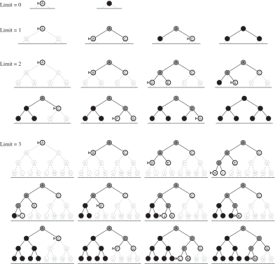
Four iterations of iterative deepening search on a binary tree.
Properties
- Time complexity
- db^{1}+(d-1)b^{2}+1b^{d}=O(b^{d})
- Space complexity
- O(bd), similar to DFS.
- Completeness
- Yes, provided the branching factor b is finite.
- Optimal: Not optimal in general.
4.6 Bidirectional search
Bidirectional search
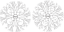
- This strategy runs two simultaneous searches:
- One from the initial state forward.
- One from the goal state backward.
- The hope is that the two searches will meet in the middle.
Properties
- Time and Space complexity: O(b^{d/2})
- Goal test: Checks whether the frontiers of the two searches intersect.
- Optimality: Generally not optimal.
- While it sounds attractive, what is the tradeoff?
- The space requirement for the frontiers of at least one search is significant.
- It is not easy to search backward (predecessors are required).
- This is difficult if there are multiple goals.
- It is especially difficult if the goal is an abstract description (e.g., “no queen attacks another queen”).
Comparing uninformed search strategies
| Criterion | Breadth-First | Uniform-Cost | Depth-First | Depth-Limited | Iterative Deepening | Bidirectional |
|---|---|---|---|---|---|---|
| Complete | Yesa | Yesa,b | No | No | Yesa | Yesa,d |
| Time | O(b^{d}) | O(b^{1+\left\lfloor \frac{C^{**}}{\epsilon}\right\rfloor }) | O(b^{m}) | O(b^{l}) | O(b^{d}) | O(b^{\frac{d}{2}}) |
| Space | O(b^{d}) | O(b^{1+\left\lfloor \frac{C^{**}}{\epsilon}\right\rfloor }) | O(bm) | O(bl) | O(bd) | O(b^{\frac{d}{2}}) |
| Optimal | Yesc | Yes | No | No | Yesc | Yesc,d |
Evaluation of tree-search strategies. b is the branching factor; d is the depth of the shallowest solution; m is the maximum depth of the search tree; l is the depth limit. Superscript caveats are as follows:a complete if b is finite;b complete if step costs \geq\epsilon for positive \epsilon;c optimal if step costs are all identical;d if both directions use breadth-first search.