6 Local Search
Optimization problems
- In many optimization problems, path is irrelevant; the goal state itself is the solution
- “Pure optimization” problems
- All states have an objective function
- Goal is to find state with max (or min) objective value
- Does not quite fit into path-cost/goal-state formulation
- Local search can do quite well on these problems.
- Then state space = set of “complete” configurations
- find optimal configuration, e.g., TSP
- find configuration satisfying constraints, e.g., timetable
Local search algorithms
- Local search
- Keep track of single current state
- Move only to neighboring states
- Ignore paths
- Advantages:
- Use very little memory
- Can often find reasonable solutions in large or infinite (continuous) state spaces.
State-space landscape
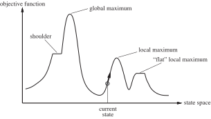
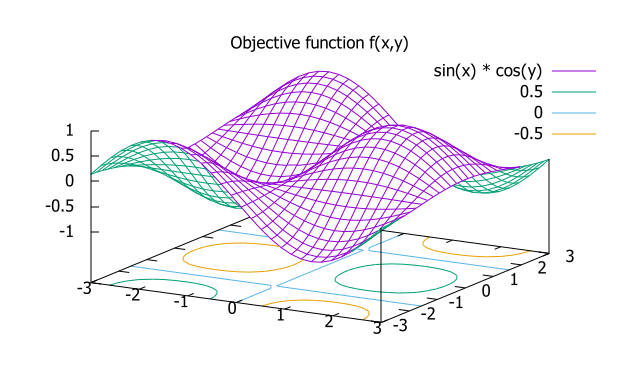
An useful landscape has both “location” (defined by the state) and “elevation’” (defined by the value of the heuristic cost function or objective function)
A one-dimensional state-space landscape in which elevation corresponds to the objective function
6.1 Hill-climbing Search
Hill-climbing Search
- The hill-climbing search algorithm (steepest-ascent version) is simply a loop that continually moves in the direction of increasing value (uphill). It terminates when it reaches a “peak” where no neighbor has a higher value.
- The algorithm does not maintain a search tree, so the data structure for the current node need only record the state and the value of the objective function.
- Hill climbing does not look ahead beyond the immediate neighbors of the current state
Algorithm
function Hill-Climbing(problem) returns a state that is a local maximum

  current ← Make-Node(problem.Initial-State)

  loop do
    neighbor ← a highest-valued successor of current
    if neighbor.Value ≤ current.Value then return current.State
current ← neighbor- At each step the current node is replaced by the best neighbor; in this version, that means the neighbor with the highest Value, but if a heuristic cost estimate h is used, we would find the neighbor with the lowest h.
- Hill-climbing algorithms typically choose randomly among the set of best successors if there is more than one.
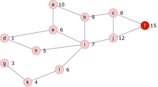
Illustration
- Find a state with the highest value.
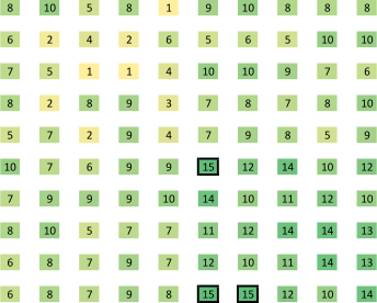
Example
- Find a state with the highest value in a grid problem.
Knapsack Problem
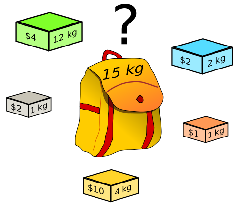
- Configurations: Any combination of objects inside the knapsack
- Initial configuration: Empty knapsack
- Actions: Put objects in and take objects from the knapsack
- Best configuration: A configuration with \max\sum value_{i}
8-queens Problem
- Complete-state formulation
- All 8 queens on the board, one per column
- Successor function
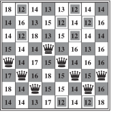
- Move a single queen to another square in the same column 8\times7=56 successors
- Heuristic cost function h(n)
- The number of pairs of queens that are attacking each other
- Global minimum has h(n)=0
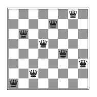
- (a) An 8-queens state with heuristic cost estimate h=17, showing the value of h for each possible successor obtained by moving a queen within its column. The best moves are marked. (b) A local minimum in the 8-queens state space; the state has h=1 but every successor has a higher cost. It takes just 5 steps from state (a) to state (b)
Problems
- Hill climbing often gets stuck for the following reasons:
- Local maxima: a local maximum is a peak that is higher than each of its neighboring states but lower than the global maximum
- Ridges: ridges result in a sequence of local maxima that is very difficult for greedy algorithms to navigate.
- Plateaux: a plateau is a flat area of the state-space landscape.
- In each case, the algorithm reaches a point at which no progress is being made. Starting from a randomly generated 8-queens state, hill climbing gets stuck 86% of the time, solving only 14% of problem instances.
- It takes 4 steps on average for each successful instance and 3 for each failure
Possible solution
- If no uphill (downhill) moves, allow sideways moves in hope that algorithm can escape local maximum
- A limit on the possible number of sideways moves required to avoid infinite loops
- 8-queens problem
- Allow sideways moves up to 100 \to percentage of problem instances solved raises from 14 to 94%
- It takes 21 steps on average for each successful instance and 64 for each failure
Variants of hill climbing
- Stochastic hill climbing
- Choose at random from among the uphill moves with a probability of selection varied with the moves’ steepness
- Usually converge more slowly than steepest ascent, but find better solutions in some cases
- First-choice hill climbing
- Generate successors randomly until better than the current state
- Good strategy when a state has many successors (e.g., thousands)
- Random-restart hill climbing: “If at first you don’t succeed, try, try again.”
- A series of hill-climbing searches from randomly generated initial states until a goal is found.
- If each hill-climbing search has a probability p of success, then the expected number of restart 1/p
- Random-walk hill climbing: At each step do one of the two
- Greedy: With probability p move to the neighbor with largest value
- Random: With probability 1-p move to a random neighbor
6.2 Simulated Annealing
Simulated Annealing
- Simulated Annealing = physics inspired twist on random walk
- A metal alloy or dissolution is heated at high temperatures and progressively cooled in a controlled way
- If the cooling process is adequate the minimal state of energy of the system is achieved (global minimum)

Algorithm
function Simulated-Annealing(problem, schedule) returns a solution state

inputs: problem, a problem
        schedule, a mapping from time to "temperature"

  current ← Make-Node(problem.Initial-State)
  for t=1 to infinity do
    T ← schedule(t)
    if T = 0 then return current
    next ← a randomly selected successor of current
    DeltaE ← next.Value - current.Value
    if DeltaE > 0 then current ← next
    else current ← next only with probability exp(DeltaE / T)
Physical Interpretation of Simulated Annealing
- A Physical Analogy:
- imagine letting a ball roll downhill on the function surface \tothis is like hill-climbing (for minimization)
- now imagine shaking the surface, while the ball rolls, gradually reducing the amount of shaking \to this is like simulated annealing
- Annealing = physical process of cooling a liquid or metal until particles achieve a certain frozen crystal state
- free variables are like particles
- seek “low energy” (high quality) configuration
- slowly reducing temp. T with particles moving around randomly
TSP Problem
- Given a list of cities and the distances
- What is the shortest possible route \{(x_{1},y_{1}),...,(x_{n},y_{n})\} that visits each city exactly once and returns to the origin city?
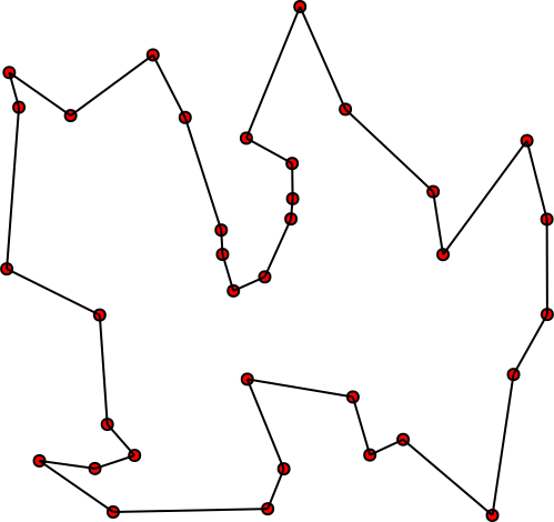
Intial a list of cities
An energy function (sum of the distance among the cities, following the order in the list)
f=\sum_{i=1}^{n}\sqrt{(x_{i}-x_{i+1})^{2}+(y_{i}-y_{i+1})^{2}}
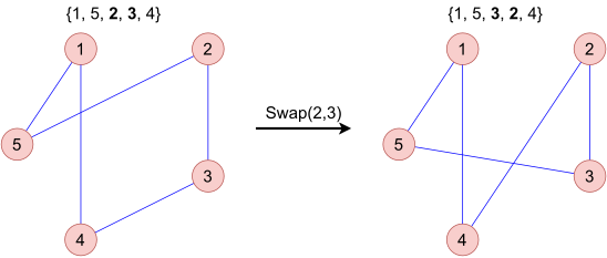
Action: swap two cities
6.3 Local Beam Search
Local Beam Search
Keep track of k states rather than just one (extreme reaction to memory problems)
Begin with k randomly generated states
At each step, all successors of all k tates are generated
If any of successors is goal \to finished
Else select k best from successors and repeat
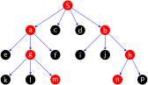
Not the same as k random-start searches run in parallel!
In its simplest form, local beam search can suffer from a lack of diversity among the k states
- They can quickly become concentrated in a small region of the state space \to an expensive version of hill climbing
Stochastic beam search
- Choose k successors at random, with the probability of choosing a given successor being an increasing function of its value

6.4 Genetic Algorithms
Genetic algorithms
A genetic algorithm (or GA) is a variant of stochastic beam search in which successor states are generated by combining two parent states rather than by modifying a single state.
The analogy to natural selection is the same as in stochastic beam search, except that now we are dealing with sexual rather than asexual reproduction.
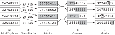
The GA begins with a set of k randomly generated states, called the population.
Each state is rated by the objective function, called the fitness function.
- Higher values for better state
Produce the next generation by “simulated evolution”
- Random selection
- Crossover
- Random mutation
Algorithm
function Genetic-Algorithm(population, Fitness-Fn) returns an individual

inputs: population, a set of individuals
        Fitness-Fn, a function that measures the fitness of an individual

  repeat
    new_population ← empty set
    for i = 1 to SIZE(population) do
      x ← Random-Selection(population, Fitness-Fn)
      y ← Random-Selection(population, Fitness-Fn)
      child ← Reproduce(x, y)
      if (small random probability) then child ← Mutate(child)
      add child to new_population
    population ← new_population
  until some individual is fit enough, or enough time has elapsed
  return the best individual in population, according to Fitness-Fn

function Reproduce(x, y) returns an individual

inputs: x, y, parent individuals

  n ← Length(x);
  c ← random number from 1 to n
  return Append(SubString(x, 1, c), SubString(y, c+1, n))
Illustration
- Representation of Individuals
- Each state, or individual, is represented as a string over a finite alphabet – most commonly, a string of 0s and 1s.
- Alternatively, the state could be represented as 8 digits, each in the range from 1 to 8.
- The genetic algorithm, illustrated for digit strings representing 8-queens states. The initial population in (a) is ranked by the fitness function in (b), resulting in pairs for mating in (c). They produce offspring in (d), which are subject to mutation in (e).
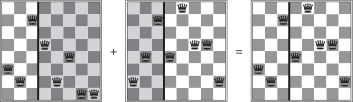
- The 8-queens states corresponding to the first two parents in Figure 3(c) and the first offspring in Figure 3(d). The shaded columns are lost in the crossover step and the unshaded columns are retained.
6.5 Local Search in Continuous Spaces
Optimization of Continuous Functions
Discrete environments: Use hill-climbing
Continuous environments: Use gradient descent
Example
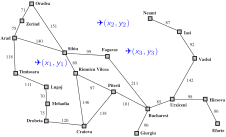
- Suppose we want to site three airports in Romania:
- 6-D state space defined by (x_{1},y_{2}), (x_{2},y_{2}), (x_{3},y_{3})
- Objective function f(\boldsymbol{x})=f(x_{1},y_{2},x_{2},y_{2},x_{3},y_{3}) = sum of squared distances from each city to nearest airport
Gradient descent
Discretization methods turn continuous space into discrete space
- E.g., empirical gradient considers \pm\delta change in each coordinate
Gradient descent methods using \nabla f=\left(\frac{\partial f}{\partial x_{1}},\frac{\partial f}{\partial y_{1}},\frac{\partial f}{\partial x_{2}},\frac{\partial f}{\partial y_{2}},\frac{\partial f}{\partial x_{3}},\frac{\partial f}{\partial y_{3}}\right)
Init \boldsymbol{x}\gets\boldsymbol{x}_{0}
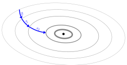
To reduce f, update \boldsymbol{x} \boldsymbol{x}\leftarrow\boldsymbol{x}-\eta\nabla f where \eta is learning rate (0<\eta<1)
Newton–Raphson methods update \boldsymbol{x} \boldsymbol{x}\leftarrow\boldsymbol{x}-\eta H^{-1}\nabla f where H is a Hesian matrix
H=\left(\begin{array}{cccc} \frac{\partial^{2}f}{\partial x_{1}\partial x_{1}} & \frac{\partial^{2}f}{\partial x_{1}\partial x_{2}} & \cdots & \frac{\partial^{2}f}{\partial x_{1}\partial x_{n}}\\ \frac{\partial^{2}f}{\partial x_{2}\partial x_{1}} & \frac{\partial^{2}f}{\partial x_{2}\partial x_{2}} & \cdots & \frac{\partial^{2}f}{\partial x_{2}\partial x_{n}}\\ \vdots & \vdots & \ddots & \vdots\\ \frac{\partial^{2}f}{\partial x_{n}\partial x_{1}} & \frac{\partial^{2}f}{\partial x_{n}\partial x_{2}} & \cdots & \frac{\partial^{2}f}{\partial x_{n}\partial x_{n}} \end{array}\right)
x_{i} approach to the optimal point
6.6 Searching With Nondeterministic Actions
The erratic vacuum world
In the erratic vacuum world, the Suck action works as follows:
- When applied to a dirty square the action cleans the square and sometimes cleans up dirt in an adjacent square, too.
- When applied to a clean square the action sometimes deposits dirt on the carpet.
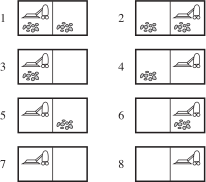
- The eight possible states of the vacuum world; states 7 and 8 are goal states.
AND–OR search trees
In this problem, a Results function that returns a set of possible outcome states
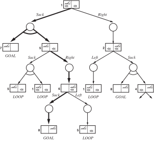
The solution to the problem is not a sequence but a contingency plan (also known as a strategy) that specifies what to do depending on what percepts are received
The first two levels of the search tree for the erratic vacuum world. State nodes are OR nodes where some action must be chosen. At the AND nodes, shown as circles, every outcome must be handled, as indicated by the arc linking the outgoing branches. The solution found is shown in bold lines.
Algorithm
function And-Or-Graph-Search(problem) returns a conditional plan, or failure
  Or-Search(problem.Initial-State, problem, empty set)

function Or-Search(state, problem, path) returns a conditional plan, or failure
  if problem.Goal-Test(state) then return the empty plan
  if state is on path then return failure
  for each action in problem.Actions(state) do
    plan ← And-Search(Results(state, action), problem, [state | path])
    if plan ≠ failure then return [action | plan]
  return failure

function And-Search(states, problem, path) returns a conditional plan, or failure
  for each s_i in states do
    plan_i ← Or-Search(s_i, problem, path)
    if plan_i = failure then return failure
  return [if s_1 then plan_1
          else if s_2 then plan_2
          else if ...
          else if s_{n-1} then plan_{n-1}
          else plan_n]