7 Constraint Satisfaction Problems
7.1 Defining Constraint Satisfaction Problems
Constraint Satisfaction Problems
- In standard search problem, state is a “black box”
- A constraint satisfaction problem (CSP) use a factored representation for each state.
- State = a set of variables and each of which has a value
- Solution = each variable has a value that satisfies all constraints on that variable
- Take advantage of the structure of states
- General-purpose rather than problem-specific heuristics
- Identify combinations of variable-value that violate the constraints \to eliminate large portions of the search space all at once
- Solutions to complex problems
A constraint satisfaction problem consists of three components, \mathcal{X}, \mathcal{D}, and \mathcal{C}:
\mathcal{X} is a set of variables, \{ X_{1},\ldots,X_{n} \}
\mathcal{D} is a set of domains, \{ D_{1},\ldots,D_{n} \}
- Each domain D_{i} consists of a set of allowable values, \{ v_{1},\ldots,v_{k}\} for variable X_{i}
\mathcal{C} is a set of constraints that specify allowable combinations of values.
Each constraint C_{j} consists of a pair \langle scope,rel \rangle, where scope is a tuple of variables that participate in the constraint and rel is a relation that defines the values that those variables can take on
- Constraint graph: nodes are variables, arcs show constraints
- CSP algorithms use the graph structure to speed up search
State Space And Solution
- Each state in a CSP is defined by an assignment of values to some or all of the variables, { X_{i}=v_{i},X_{j}=v_{j},\ldots}
- An assignment that does not violate any constraints is called a consistent or legal assignment.
- A complete assignment is one in which every variable is assigned
- A partial assignment is one that assigns values to only some of the variables.
- A solution to a CSP is a consistent, complete assignment.
We may want to solve the a problem with CSP:
- determine whether or not a solution exists
- find a solution (default)
- find all of the solutions
- count the number of solutions
- find the best solution, given some measure of model quality this is now an optimization problem
- determine whether some property of the variables holds in all solutions
Example problem: Map coloring
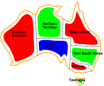
The principal states and territories of Australia. Coloring this map can be viewed as a constraint satisfaction problem (CSP). The goal is to assign colors to each region so that no neighboring regions have the same color.

The map-coloring problem represented as a constraint graph.
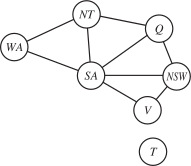
Variables: \{ WA,NT,Q,NSW,V,SA,T \}
Domains: D_{i}=\{red,green,blue\}
Constraints: adjacent regions must have different colors
\begin{align*} \mathcal{C} & =\{SA\neq WA,SA\neq NT,SA\neq Q,SA\neq NSW,SA\neq V,\\ & WA\neq NT,NT\neq Q,Q\neq NSW,NSW\neq V\} \end{align*}
There are many possible solutions to this problem, e.g.,
\begin{align*} & \{WA=red,NT=green,Q=red,NSW=green,\\ & V=red,SA=blue,T=green\} \end{align*}
Example problem: Job-shop scheduling
- We consider a small part of the car assembly, consisting of 15 tasks:
- install axles (front and back)
- affix all four wheels (right and left, front and back)
- tighten nuts for each wheel
- affix hubcaps
- inspect the final assembly.
- Some tasks must occur before another while many other tasks can go on at once.
- E.g., a wheel must be installed before the hubcap is put on
- A task takes a certain amount of time to complete.
We can represent the tasks with 15 variables:
Variables:
\begin{align*} \mathcal{X}= & \{Axle_{F},Axle_{B},\\ & Wheel_{RF},Wheel_{LF},Wheel_{RB},Wheel_{LB},\\ & Nuts_{RF},Nuts_{LF},Nuts_{RB},Nuts_{LB},\\ & Cap_{RF},Cap_{LF},Cap_{RB},Cap_{LB},\\ & Inspect\} \end{align*}
Domains: D_{i}: the value of each variable is the time that the task starts
Constraints: Assume task T_{1} and T_{2} take duration d_{1} and d_{2} to complete
- Precedence constraints: task T_{1} must occur before task T_{2}; T_{1}+d_{1}\leq T_{2}
- Disjunctive constraint: task T_{1} and task T_{2} must not overlap in time T_{1}+d_{1}\leq T_{2}\text{ or }T_{2}+d_{2}\leq T_{1}
The axles have to be in place before the wheels are put on, and it takes 10 minutes to install an axle
\begin{array}{ll} Axle_{F}+10\leq Wheel_{RF} & Axle_{F}+10\leq Wheel_{LF}\\ Axle_{B}+10\leq Wheel_{RB} & Axle_{B}+10\leq Wheel_{LB} \end{array}
For each wheel, we must affix the wheel (which takes 1 minute), then tighten the nuts (2 minutes), and finally attach the hubcap (1 minute)
\cdots
Suppose we have four workers to install wheels, but they have to share one tool that helps put the axle in place
\cdots
The inspection comes last and takes 3 minutes
\forall X\neq Inspect,X+d_{X}\leq Inspect
Finally, suppose there is a requirement to get the whole assembly done in 30 minutes \to limit the domain of all variables to
D_{j}={ 1,2,3,\ldots,27}
Example problem: 4-Queens
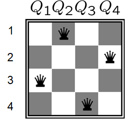
- Variables: \{Q_{1},Q_{2},Q_{3},Q_{4}\}
- Domains: D_{i}={1,2,3,4}
- Constraints:
- Q_{i}\neq Q_{j} (cannot be in same row)
- |Q_{i}-Q_{j}|\neq|i-j| (or same diagonal)
Example problem: Cryptarithmetic
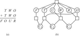
- Variables: \{F,T,U,W,R,O,C_{1},C_{2},C_{3}\}
- Domains: D_{i}=\{0,1,2,3,4,5,6,7,8,9\}
- Constraints:
- Alldiff(F,T,U,W,R,O)
- T\neq0,F\neq0
- C_{3}=F,…
Why formulate a problem as a CSP
- Provide natural representation for a wide variety of problems
- Many problems intractable in regular state-space search can be solved quickly with CSP formulation.
For example, once we have chosen \{SA=blue\} in the Australia problem.
- Search: 3^{5}=243 assignments
- CSP: 2^{5}=32 assignments
- Better insights to the problem and its solution
Varieties of CSPs
- Discrete variables and finite domains
- n variables with size d \to O(n^{d}) complete assignments
- E.g., Boolean CSPs, including Boolean satisfiability (NP-complete)
- Discrete variables and infinite domains
- E.g., job scheduling, variables are start/end times for each job
- Continuous variables
- E.g., start/end times for Hubble Telescope observations
Varieties of constraints
- Unary constraints involve a single variable, e.g., SA\neq green
- Binary constraints involve pairs of variables, e.g., SA\neq WA
- Higher-order constraints involve 3 or more variables, e.g., cryptarithmetic column constraints
- Preferences (soft constraints), e.g., red is better than green often representable by a cost for each variable assignment \rightarrow constrained optimization problems
Real-world CSPs
- Assignment problems; e.g., who teaches what class?
- Timetabling problems; e.g., which class is offered when and where?
- Hardware configuration
- Spreadsheets
- Transportation scheduling
- Factory scheduling
- Floorplanning
7.2 Backtracking Search for CSPs
CSP as Standard Search Problem
Let’s start with the straightforward, dumb approach, then fix it
States are defined by the values assigned so far
Initial state: the empty assignment, \emptyset
Successor function: assign a value to an unassigned variable that does not conflict with current assignment \implies fail if no legal assignments (not fixable!)
Goal test: the current assignment is complete
- This is the same for all CSPs!
- Every solution appears at depth n with n variables \implies use depth-first search
- Path is irrelevant, so can also use complete-state formulation
- Branching factor b=(n-\ell)d at depth \ell, hence n!d^{n} leaves!
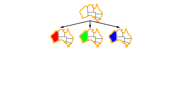
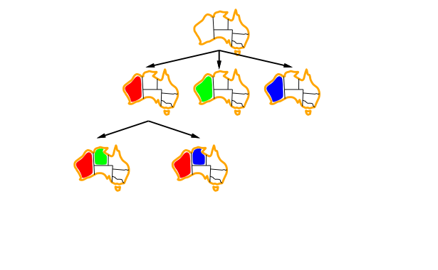
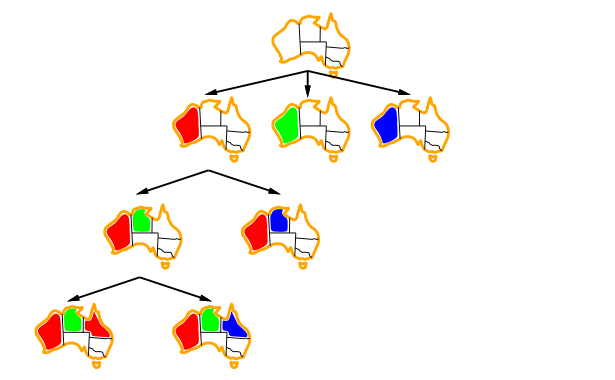
Backtracking search
- Variable assignments are commutative, i.e., [WA=red then NT=green] same as [NT=green then WA=red]
- Only need to consider assignments to a single variable at each node \implies b=d and there are d^{n} leaves
- Depth-first search for CSPs with single-variable assignments is called backtracking search
- Backtracking search is the basic uninformed algorithm for CSPs
- Can solve n-queens for n\approx25
Algorithm
function Backtracking-Search(csp) returns a solution, or failure

  return Backtrack(⌀, csp)

function Backtrack(assignment, csp) returns a solution, or failure

  if assignment is complete then return assignment
  var ← Select-Unassigned-Variable(csp)
  for each value in Order-Domain-Values(var, assignment, csp) do
    if value is consistent with assignment then
      add {var=value} to assignment
      inferences ← Inference(csp, var, value)
      if inferences ≠ failure then
        add inferences to assignment
        result ← Backtrack(assignment, csp)
        if result ≠ failure then
          return result
      remove {var=value} and inferences from assignment
  return failure
Illustration
 |
 |
 |
 |
Improving backtracking efficiency
General-purpose methods can give huge gains in speed:
- Which variable should be assigned next?
- In what order should its values be tried?
- Can we detect inevitable failure early?
- Can we take advantage of problem structure?
Minimum remaining values
The backtracking algorithm contains the line var \gets Select-Unassigned-Variable(csp)
We need a strategy for Select-Unassigned-Variable to choose the next unassigned variable in \{X_{1},X_{2},\ldots\}
- Minimum remaining values (MRV): choose the variable with the fewest legal values
- MRV usually performs better than a random/static ordering, sometimes by a factor of 1,000 or more

Degree heuristic
- Tie-breaker among MRV variables
- Degree heuristic: choose the variable with the most constraints on remaining variables

Least constraining value
The backtracking algorithm contains the line value in Order-Domain-Values(var, assignment, csp)
Given a variable, choose the least constraining value: the one that rules out the fewest values in the remaining variables
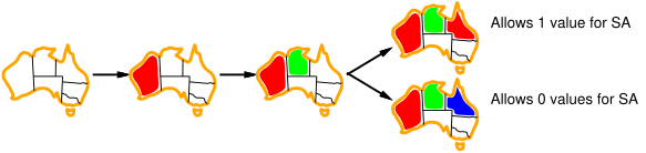
Combining these heuristics makes 1000 queens feasible
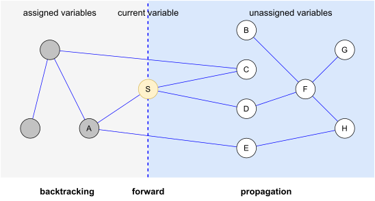
Inference: Forward checking
Idea: Keep track of remaining legal values for unassigned variables
\to Terminate search when any variable has no legal values
inferences \gets Inference(csp, var, value)
Note: Forward checking propagates information from assigned to unassigned variables, but doesn’t provide early detection for all failures!
Inference: Forward checking
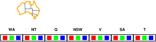
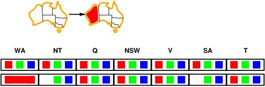
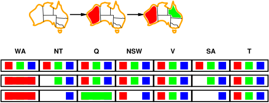
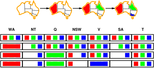
7.3 Constraint Propagation: Inference in CSPs
Constraint propagation
- Reduce the number of legal values for a variable by using constraints \to legal values for another variable also reduced
- Intertwined with search, or done as a preprocessing step
- Sometimes the preprocessing can solve the whole problem!
- Enforcing local consistency in each part of a graph causes inconsistent values to be eliminated throughout the graph
Node consistency
- A single variable is node-consistent if all the values in the variable’s domain satisfy the variable’s unary constraints
- South Australians dislike green, SA=\{red,green,blue\} \to SA=\{red,blue\}
- Eliminate all the unary constraints in a CSP by running node consistency
Arc consistency
- A variable in a CSP is arc-consistent if every value in its domain satisfies the variable’s binary constraints. More formally, X\rightarrow Y is consistent iff for every value x of X there is some allowed y
- Run as a preprocessor before the search starts or after each assignment, must be run repeatedly until no inconsistency remains.
- Trade-off
- Requires some overhead to do, but generally more effective than direct search
- Eliminate large (inconsistent) parts of the state-space more effectively than search
- Need a systematic method for arc-checking
- If Y loses a value, neighbors of Y need to be rechecked \to incoming arcs can become inconsistent again while outgoing arcs stay still
Algorithm
function AC-3(csp) returns false/true

inputs: csp, a binary CSP with components (X, D, C)
variables: queue, a queue of arcs, initially all the arcs in csp

  while queue ≠ ⌀ do
    (X_i, X_j) ← Remove-First(queue)
    if Revise(csp, X_i, X_j) then
      if size of D_i = 0 then return false
      for each X_k in X_i.Neighbors - {X_j} do
        add (X_k, X_i) to queue
  return true

function Revise(csp, X_i, X_j) returns true iff we revise the domain of X_i

  revised ← false
  for each x in D_i do
    if no value y in D_j allows (x,y) to satisfy
       the constraint between X_i and X_j then
      delete x from D_i
      revised ← true
  return revised
Illustration
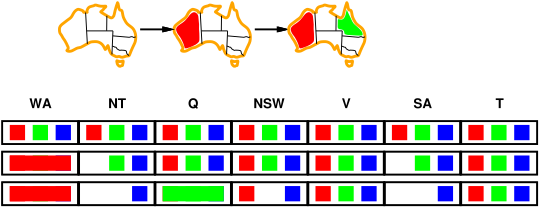
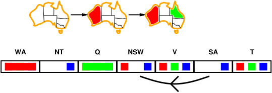
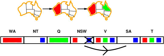
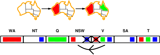
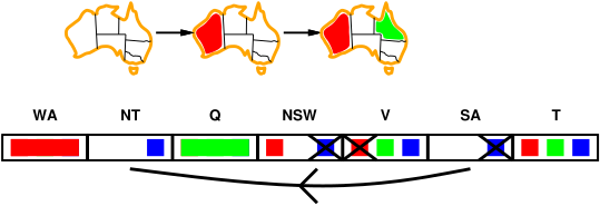
Comparison of Methods
Which constraints are tested for each method?
7.4 Local Search for CSPs
Local search for CSPs
- Complete-state formulation
- The initial state assigns a value to every variable \to violation
- The search changes the value of one variable at a time \to eliminate the violated constraints
- Min-conflicts heuristic: the minimum number of conflicts with other variables
- Min-conflicts is surprisingly effective for many CSPs.
- Million-queens problem can be solved \sim 50 steps
- Hubble Space Telescope: the time taken to schedule a week of observations down from 3 weeks to \sim 10 minutes
Algorithm
function Min-Conflicts(csp, max_steps) returns a solution of failure

inputs: csp, a constraint satisfaction problem
        max_steps, the number of steps allowed before giving up

  current ← an initial complete assignment for csp
  for i = 1 to max_steps do
    if current is a solution for csp then return current
    var ← a randomly chosen conflicted variable from csp.Variables
    value ← the value v for var that minimizes Conflicts(var, v, current, csp)
    set {var=value} in current
  return failure
Performance of min-conflicts
- Given random initial state, can solve n-queens in almost constant time for arbitrary n with high probability (e.g., n=10,000,000)
- The same appears to be true for any randomly-generated CSP except in a narrow range of the ratio R=\frac{\text{number of constraints}}{\text{number of variables}}
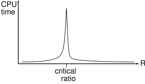
Illustration: 8-queens
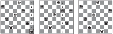
- A two-step solution using min-conflicts for an 8-queens problem. At each stage, a queen is chosen for reassignment in its column. The number of conflicts (in this case, the number of attacking queens) is shown in each square. The algorithm moves the queen to the min-conflicts square, breaking ties randomly.
Improving min-conflicts
- The landscape of a CSP under the min-conflicts heuristic usually has a series of plateaux.
- Millions of variable assignments that are only one conflict away from a solution
- Plateau search: allow sideways moves to another state with the same score
- Tabu search: keep a small list of recently visited states and forbid the algorithm to return to those states
- Simulated annealing can also be used
Constraint weighting
- Concentrate the search on the important constraints
- Each constraint is given a numeric weight, W_{i}, initially all 1.
- At each step, chooses a variable/value pair to change that has the lowest total weight of all violated constraints.
- Increase the weight of each constraint that is violated by the current assignment.
Local search in online setting
- Scheduling problems: online setting
- A week’s airline schedule may involve thousands of flights and tens of thousands of personnel assignments
- The bad weather at one airport can render the schedule infeasible.
- The schedule should be repaired with a minimum number of changes.
- Done easily with a local search starting from the current schedule
- A backtracking search with the new set of constraints usually requires much more time and might find a solution with many changes from the current schedule
7.5 The Structure of Problems
Independent subproblems
A problem CSP is decomposed into independent subproblems CSP_{i}
- Independent subproblems are identifiable as connected components of constraint graph
Tasmania and mainland are independent subproblems
If assignmen S_{i} is a solution of CSP_{i} then
S=\bigcup_{i=1}^{n} S_{i}\text{ is a solution of }CSP
Suppose a problem of n variables can be broken into independent subproblems of only c variables
- Worst-case solution cost is O(\frac{n}{c}d^{c})
- Original CSP has worst-case solution O(d^{n})
Tree-structured CSPs
A CSP is a tree-structured CSP if the constraint graph has no loops
Theorem
A tree-structured CSP can be solved in O(n\times d^{2}) time, compare to general CSPs, where worst-case time is O(d^{n})
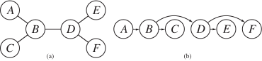
Using Topologicalsort to create an ordering of the variables such that each variable appears after its parent in the tree
(a) The constraint graph of a tree-structured CSP. (b) A linear ordering of the variables consistent with the tree with A as the root. This is known as a topological sort of the variables
Algorithm
function Tree-Csp-Solver(csp) returns a solution, or failure

inputs: csp, a CSP with components X, D, C

  n ← |X|
  assignment ← ⌀
  root ← any variable in X
  X ← Topologicalsort(X, root)
  for j = n down to 2 do
    Make-Arc-Consistent(Parent(X_j), X_j)
    if it cannot be made consistent then return failure
  for i = 1 to n do
    assignment[X_i] ← any consistent value from D_i
    if there is no consistent value then return failure
  return assignment
Nearly tree-structured CSPs
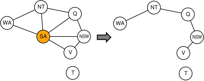
Cycle cutset: a set of variables such that the remaining constraint graph is a tree
The removal of SA makes the constraint graph to be a tree
Cutset Conditioning
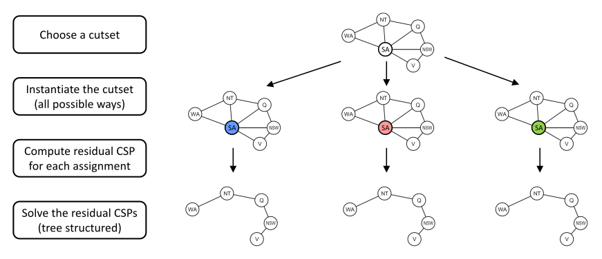
- If the cycle cutset has size c, then the total run time is O(d^{c}(n-c)d^{2})
Tree Decomposition
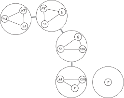
Idea: create a tree-structured graph of mega-variables
- Each mega-variable encodes part of the original CSP
- Subproblems overlap to ensure consistent solutions
A tree decomposition must satisfy the following three requirements:
- Every variable in the original problem appears in at least one of the subproblems.
- If two variables are connected by a constraint in the original problem, they must appear together (along with the constraint) in at least one of the subproblems.
- If a variable appears in two subproblems in the tree, it must appear in every subproblem along the path connecting those subproblems.
A tree decomposition of the constraint graph
The structure of values
- Consider the map-coloring problem with n colors.
- For every consistent solution, there is actually a set of n! solutions formed by permuting the color names.
- E.g., WA, NT, and SA must all have different colors, but there are 3! ways to assign the three colors to these three regions.
- Symmetry-breaking constraint: Impose an arbitrary ordering constraint that requires the values to be in alphabetical order.
- E.g., NT < SA < WA \toonly one solution possible {NT = blue, SA = green, WA = red}